2. Introduction into the Mathematical Methods
Covariance and correlation (1/2)
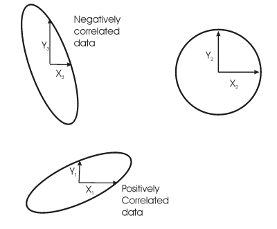
We have seen that data can be correlated so that an increase in one parameter will normally be matched by an increase in the second parameter. In these cases the scattergram shows the structure of a line going diagonal from bottom left to top right of the plot. How do we measure this correlation, and how do we display it?
To do this we will adapt the variance equation that you met in the chapter on measures of spread and call it covariance. From the covariance we will derive the correlation.
You will recall that the variance equation is:
In a similar way, the sample covariance between variables x and y is given by:
Now we can construct these variance and covariance values as a matrix:
In this matrix there are but two variables (x and y) and so it forms a (2,2) array. You can do this for any number of variables, so for n variables you would derive an (n,n) covariance array. In a covariance array, as you can see, the diagonal elements from the top left to the bottom right, are the variances, and the values off this diagonal are the covariance values.
The correlation between x and y is given by:
So we can construct the correlation matrix by dividing the values in each row by the standard deviation in that row and then dividing the values in each column by the standard deviation value for that column. For two variables we get

