Supplement 1.7: Radiation quantities and radiometry (4/5)

The radiant intensity ... continued from the previous page

For an isotropic emitter with direction-independent beam intensity, the integral can be solved. In the case of a conical solid angle, as shown in the diagram in the left-hand column on the previous page, but oriented towards the zenith, the azimuth angle $φ$ varies from 0 to $2 π$ . The zenith angle $ϑ$ varies from 0 to half the aperture angle $ϑ'$ :

Φ = I \int_{ϑ = 0}^{ϑ'} \int_{φ = 0}^{2 π} sin ϑ d ϑ d φ = I \cdot 2 π (1 - cos ϑ')

This solution is an alternative to the calculation in the example Efficiency of a lens collimator on the previous page.

Task 2: Isotropic emitters ↓

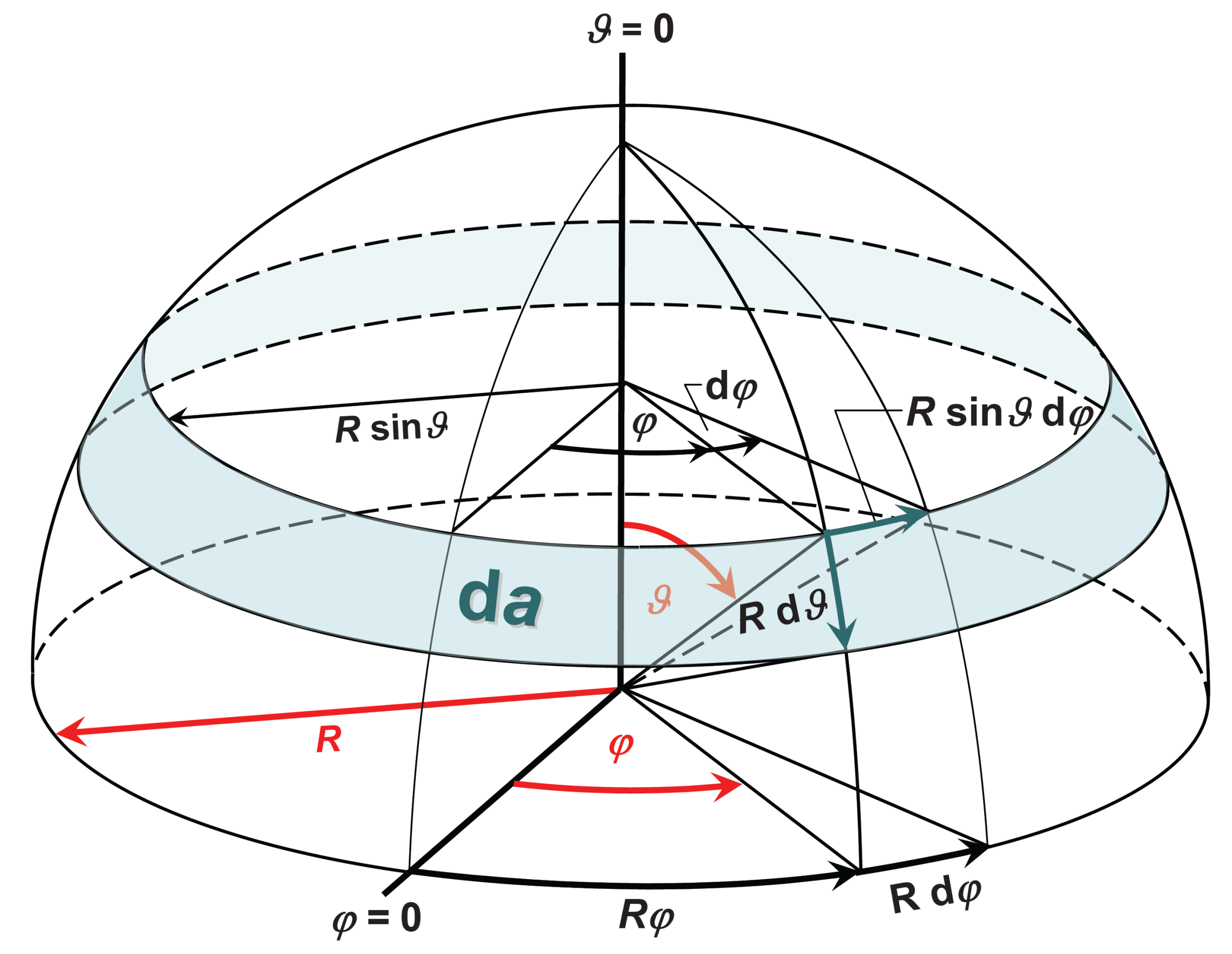
For anisotropic emitters whose emission is symmetrical about an axis, the integral can be partially solved. To do this, we consider the following graph, which shows an axially symmetrical solid angle around the vertical axis (the zenith axis) and appears as a band wrapped around the hemisphere. This solid angle, which is also differential, is:

d Ω = \frac{d a}{R^{2}} = \int_{φ = 0}^{2 π} sin ϑ d ϑ d φ = 2 π sin ϑ d ϑ

By assuming a radiant intensity $I (ϑ)$ that depends only on the zenith angle ϑ, the emission can be integrated over the azimuth angle φ:

Φ = \int_{ϑ_{1}}^{ϑ_{2}} \int_{φ = 0}^{2 π} I (ϑ) sin ϑ d ϑ d φ = 2 π \int_{ϑ_{1}}^{ϑ_{2}} I (ϑ) sin ϑ d ϑ

Equations ↓

Integration over the azimuth angle φ from 0 to

2 π

results in a band around the sphere under the zenith angle ϑ with a width Rdϑ. Due to the differential width, this band is also a differential surface element da.

Task 3: Anisotropic emitters ↓

The axially symmetrical radiant intensity of a lamp is given by

I (ϑ) = \frac{1}{2} I (ϑ = 0) (1 + cos ϑ)

Please sketch the distribution of the radiant intensity over the zenith angle ϑ from 0 to 180°.
Calculate the total radiant power emitted as a function of the radiant intensity for ϑ = 0.

Check your results on this page!

A special type of anisotropic emitter is the cosine emitter or Lambert emitter, named after the mathematician and physicist Johann Heinrich Lambert (1728–1777). These emitters are discussed in Supplement 1.8.

Methods for measuring radiant intensity are presented in the section on radiance.

Understanding Spectra from the Earth

Supplement 1.7: Radiation quantities and radiometry (4/5)

The radiant intensity ... continued from the previous page