Supplement 2.1: Point Clouds and Linear Regression Lines (1/3)

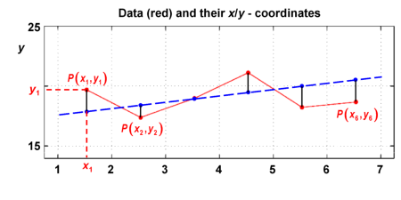
A point cloud is considered, with i=1...n data points $P(x_i,y_i)$ , where n is a natural number (left graph below). We search for a regression line which best approximates the distribution of data points. For this, the equation of a straight line, shown as blue broken line in the diagrams,

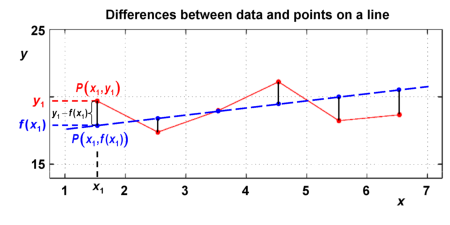
is investigated, and in particular the points $P(x_i,f(x_i))$ on that line having the same x coordinates as the data points (right graph below, click on the graph titles to switch sides).

Point cloud P(x_i,y_i) Straight line and projected points P(x_i,f(x_i))

The difference between data points and points on the line having the same x values is $y_i-f(x_i)$. These differences, shown in the graph below for points $P(x_1,y_1)$ and $P\left(x_1,f(x_1)\right)$ as an example, provide a means to find the best-fit line that represents the data points. This best-fit line should indeed have minimum differences to the data points!

Alternatively, one could also investigate the differences between data points and points on the line having the same y values. This would lead to a regression analysis with respect to y.

In the following equations, we investigate the regression analysis with respect to x.

It would not be useful to simply add up the differences and find a minimum by varying the line parameters since the differences are positive and negative. Instead, we get rid of the + or - sign of differences by squaring them, and we calculate the mean square deviation

here:                           $S=\frac{{\left(y_1-f(x_1)\right)}^2+\mathrm{...}+{\left(y_6-f(x_6)\right)}^2}{6}$

Substituting $f(x_i)$ with $f(x_i)=a{x}_i+b$ yields:

where a is the slope and b is the intercept of the straight line.

The centroid of data points

To find the best fit straight line, parameters a and b of the straight line shall be chosen such that the squared mean deviation

is a minimum. For this, we calculate the derivative of S and set it to zero.

However, S depends on two variables, a and b. Therefore we calculate the derivative in two steps. In a first step we differentiate S with respect to b and keep a as a constant. Second, we differentiate S with respect to a and keep b as a constant. (In advanced calculus, S is called a function of two variables, and we calculate the partial derivatives of S with respect to a und b)

Differentiation with respect to b yields:

With              $\frac{1}{n}\sum _{i=1}^n{y}_i=\overline{y}\frac{1}{n}\sum _{i=1}^n{x}_i=\overline{x}\frac{1}{n}\sum _{i=1}^{n}b=b$

where $\overline{x}$ and $\overline{y}$ are the arithmetic mean of the $x_i$ and $y_i$ coordinates, it follows:

The minimum of $S(b)$ follows from setting $S\text{'}(b)=0$, and one obtains:

This looks like the equation of a straight line. However, $\overline{x}$ and $\overline{y}$ are point coordinates (the mean values). The point $P(\overline{x},\overline{y})$ is the arithmetic mean of the points $P(x_i,y_i)$, denoted as their centroid.

Centroid $P(\overline{x},\overline{y})$ of the data points.