Supplement 2.1: Point Clouds and Linear Regression Lines (3/3)

The correlation coefficient

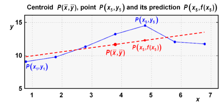
We consider a number of data points $P (x_{i}, y_{i})$ , with i=1, ..., n. The points are defined by a set of n couples of features $x_{i}$ and $y_{i}$ . As already shown, one can calculate the centroid of the point cloud and the best-fit straight line. We are interested in a quantity which gives evidence of the deviation of the points from the best-fit line. As an example we focus on point $P (x_{5}, y_{5})$ in the graph below, and on its position $P (x_{5}, f (x_{5}))$ as predicted by the best-fit line.

Water temperatures in October near Spiekeroog island (blue dots), best-fit line (red broken line) and centroid

P (\bar{x}, \bar{y})

. Point

P (x_{5}, y_{5})

is compared with its position predicted by the best-fit line

P (x_{5}, f (x_{5}))

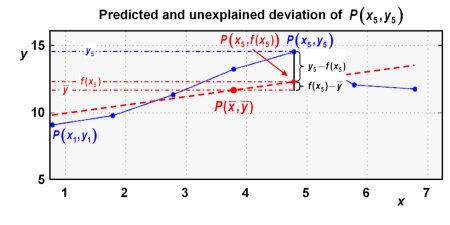
The position of $P (x_{5}, y_{5})$ is now explained in two steps, as illustrated in the graph below:

the location of point $P (x_{5}, f (x_{5}))$ with the same x=x₅, predicted by the best-fit line: $f (x_{5}) - \bar{y}$
(deviation predicted by the best-fit line)
the deviation of $P (x_{5}, y_{5})$ with respect to $P (x_{5}, f (x_{5}))$ : $y_{5} - f (x_{5})$
(unexplained deviation)

Explanation of the position of

P (x_{5}, y_{5})

in two steps: part predicted through the best-fit line (lower bracket), and unexplained part (upper bracket).

This concept can be applied with all points of the point cloud, in order to represent their deviations from the best-fit line.

The quantity which gives evidence of the quality in which way the best-fit line represents the point cloud is the correlation coefficient r, defined as follows:

r = \frac{square root of the predicted squared deviations}{square root of the total squared deviations}

r = \frac{\sqrt{\frac{1}{n} \sum_{i = 1}^{n} {(f (x_{i}) - \bar{y})}^{2}}}{\sqrt{\frac{1}{n} \sum_{i = 1}^{n} {(y_{i} - \bar{y})}^{2}}} = \frac{\sqrt{\sum_{i = 1}^{n} {(f (x_{i}) - \bar{y})}^{2}}}{\sqrt{\sum_{i = 1}^{n} {(y_{i} - \bar{y})}^{2}}}

The linear correlation coefficient

The equation of the correlation coefficient given in chapter 2 on page Linear Regression Analysis (3/3) differs from the equation given in the left column. It holds for best-fit straight lines only (hence: linear correlation coefficient), while the equation given in the left column is also valid for curved best-fit lines.

The equation for the linear correlation coefficient can be obtained by squaring the equation given in the left column, and by repacing $f (x_{i}) - \bar{y}$ with $a (x_{i} - \bar{x})$ :

r^{2} = \frac{a^{2} \sum_{i = 1}^{n} {(x_{i} - \bar{x})}^{2}}{\sum_{i = 1}^{n} {(y_{i} - \bar{y})}^{2}}

Using the slope a given on the preceeding page yields:

r^{2} = \frac{{(\sum_{i = 1}^{n} (x_{i} - \bar{x}) (y_{i} - \bar{y}))}^{2}}{{(\sum_{i = 1}^{n} {(x_{i} - \bar{x})}^{2})}^{2}} \frac{\sum_{i = 1}^{n} {(x_{i} - \bar{x})}^{2}}{\sum_{i = 1}^{n} {(y_{i} - \bar{y})}^{2}}

This can be simplified by cancelling:

r^{2} = \frac{{(\sum_{i = 1}^{n} (x_{i} - \bar{x}) (y_{i} - \bar{y}))}^{2}}{\sum_{i = 1}^{n} {(x_{i} - \bar{x})}^{2} \sum_{i = 1}^{n} {(y_{i} - \bar{y})}^{2}}

It follows by taking the square root:

r = \frac{| \sum_{i = 1}^{n} (x_{i} - \bar{x}) (y_{i} - \bar{y}) |}{\sqrt{\sum_{i = 1}^{n} {(x_{i} - \bar{x})}^{2} \sum_{i = 1}^{n} {(y_{i} - \bar{y})}^{2}}}

Omitting the absolute value bars,

r = \frac{\sum_{i = 1}^{n} (x_{i} - \bar{x}) (y_{i} - \bar{y})}{\sqrt{\sum_{i = 1}^{n} {(x_{i} - \bar{x})}^{2} \sum_{i = 1}^{n} {(y_{i} - \bar{y})}^{2}}}

allows the correlation coefficient to take on negative values: usually r has the same sign as a.

It is advantageous with this equation that it includes the coordinates of the centroid and the data points only. The equation given in the left column requires also the coordinate valus of the best fit line.

Time Series

Supplement 2.1: Point Clouds and Linear Regression Lines (3/3)

The correlation coefficient

The linear correlation coefficient