2. Working with Time Series

Linear regression analysis (2/3)

Step 2: Calculating the slope cont.

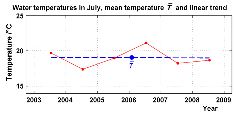
We consider the July temperatures, again converted to points $P (x_{i}, y_{i})$ with i=1, ..., 6, as given in the data table.

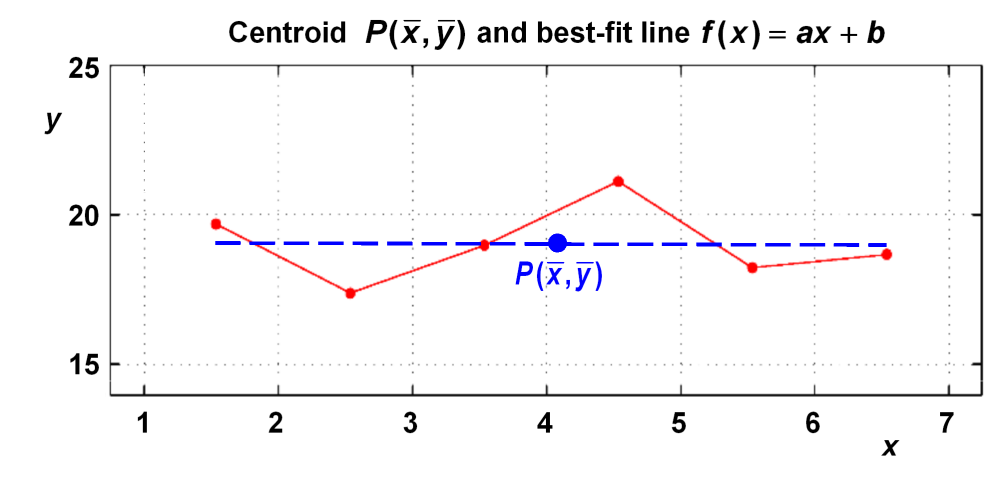
We already calculated the centroid $P (\bar{x}, \bar{y})$ of the data points which is at $\bar{x} = 4.08$ and $\bar{y} = 19.01$ .

The slope a of the best-fit line

f (x) = a x + b

which has the smallest distance to the data points is calculated according to the method of the least squares fit to:

a = \frac{\sum_{i = 1}^{n} (x_{i} - \bar{x}) (y_{i} - \bar{y})}{\sum_{i = 1}^{n} {(x_{i} - \bar{x})}^{2}}

Again, you will find this relation derived in supplement 1 in detail. With our temperature data one calculates:

a = \frac{(x_{1} - \bar{x}) (y_{1} - \bar{y}) + ... + (x_{6} - \bar{x}) (y_{6} - \bar{y})}{{(x_{1} - \bar{x})}^{2} + ... + {(x_{6} - \bar{x})}^{2}} = - 0.0117

We use now the point-slope form to calculate the best-fit straight line:

f (x) - \bar{y} = a (x - \bar{x})

Step 3: Calculating the intercept

The intercept b of the best-fit line is calculated by re-arranging the equation above:

b = \bar{y} - a \bar{x} = 19.01

Finally, the best-fit line becomes:

f (x) = - 0.0117 x + 19.01

Data points, their centroid

P (\bar{x}, \bar{y})

and linear best-fit line

f (x) = a x + b

Converted to seawater temperatures in July, the best-fit line reads:

T (t) = - 0.0117 t + 42.50

where T is the temperature in °C and t is the calendar year.

Seawater temperature near Spiekeroog in July 2003-2008, mean July temperature in these years, and linear temperature trend.